# Chapter 4: Bivariate analysis of qualitative variables

---

## Learning goals

- Dependent/independent variable

- Apply suitable analysis techniques for each combination of measurement
  levels

- Contingency tables and Cramér's $V$

- Visualization

-v-

## Overview: bivariate analysis techniques

-v-

## Overview: bivariate analysis - visualization

-v-

## Bivariate analysis

- ...is determining whether there is an association between two
  stochastic variables ($X$ and $Y$).

- **Association** = you can predict (to some extent) the value of $Y$
  from the value of $X$

- $X$: Independent variable

- $Y$: Dependent variable

- **Important!** Finding an association does **NOT** imply a causal relation!

-v-

## Example research questions

- Is there a difference in taste preference between two beverage brands?

- Is there a difference in spending at the campus restaurant between
  students and staff?

- Do smokers die more often of lung cancer than non-smokers?

- Do men and women have a different opinion on a survey question?

- ...

We will use [data/rlanders.csv](https://github.com/HoGentTIN/dsai-labs/blob/main/data/rlanders.csv) from the Github repo for lab assignments
to explore the last question.

---

# Contingency tables

-v-

## Contingency tables (cross-tabs)

See Python example code in [4.01-chi-squared.ipynb](https://github.com/HoGentTIN/dsai-labs/blob/main/4-bivariate-qual/4.01-chi-squared.ipynb)

|                   | **Female** | **Male** |
| ----------------: | ---------: | -------: |
| Strongly disagree |          0 |        4 |
|          Disagree |         17 |       45 |
|           Neutral |         23 |       91 |
|             Agree |         12 |       53 |
|    Strongly agree |          0 |        5 |

---

# Visualization

-v-

## Clustered bar plot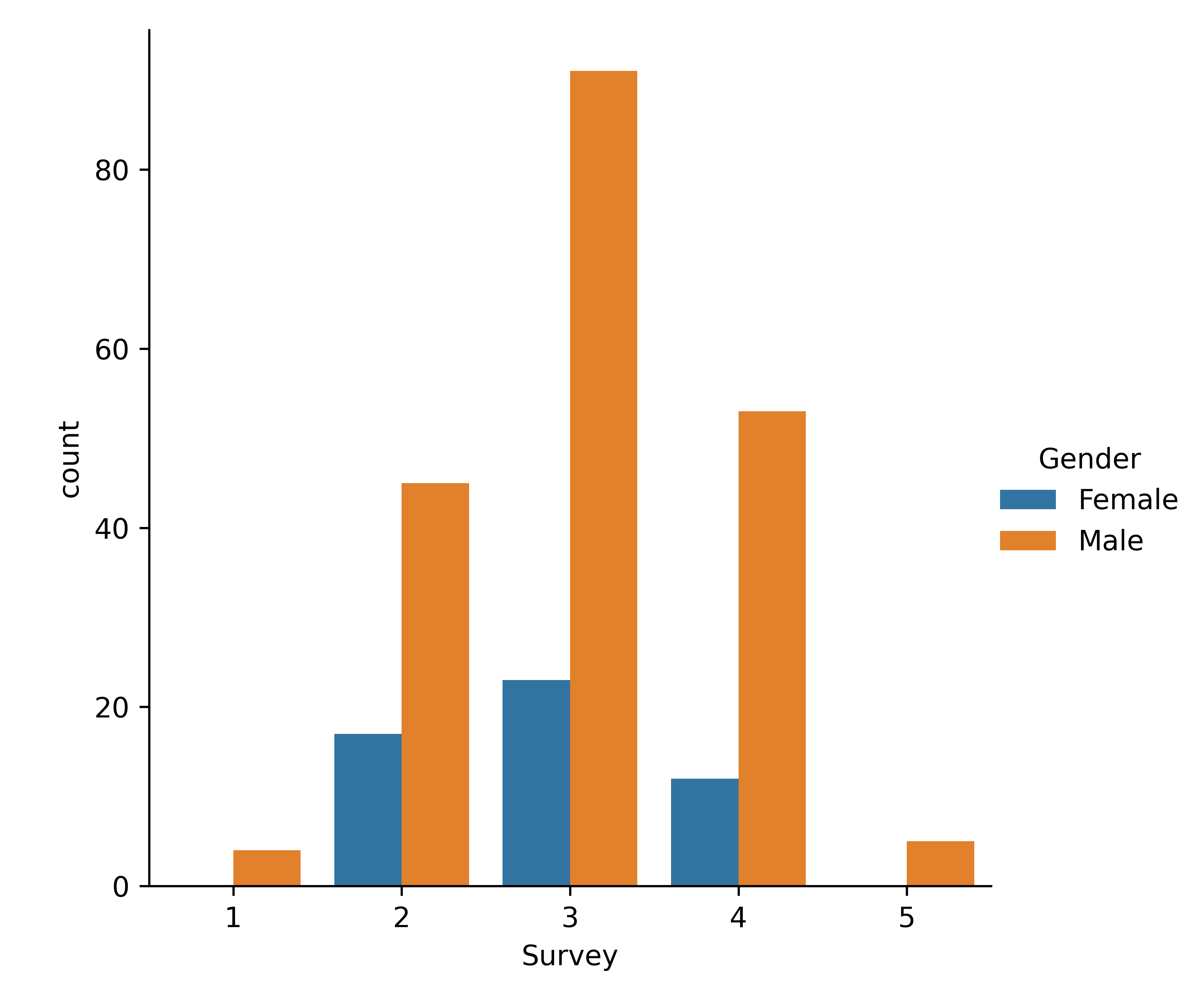

![A clustered bar plot](./img/4/gender-survey-bar.png)

-v-

## Stacked bar plot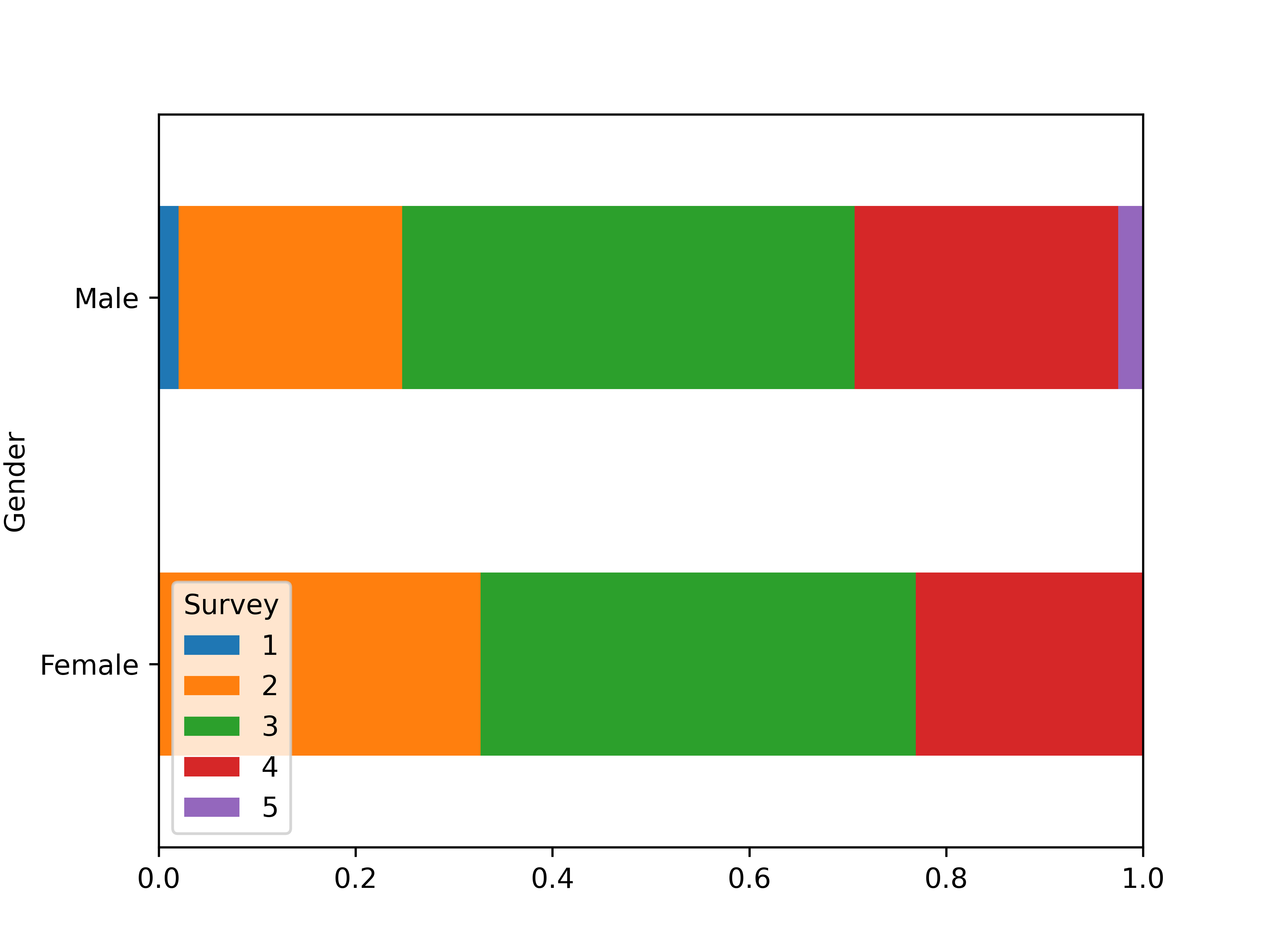

![A stacked bar plot](./img/4/gender-survey-stacked.png)

-v-

## Mosaic plot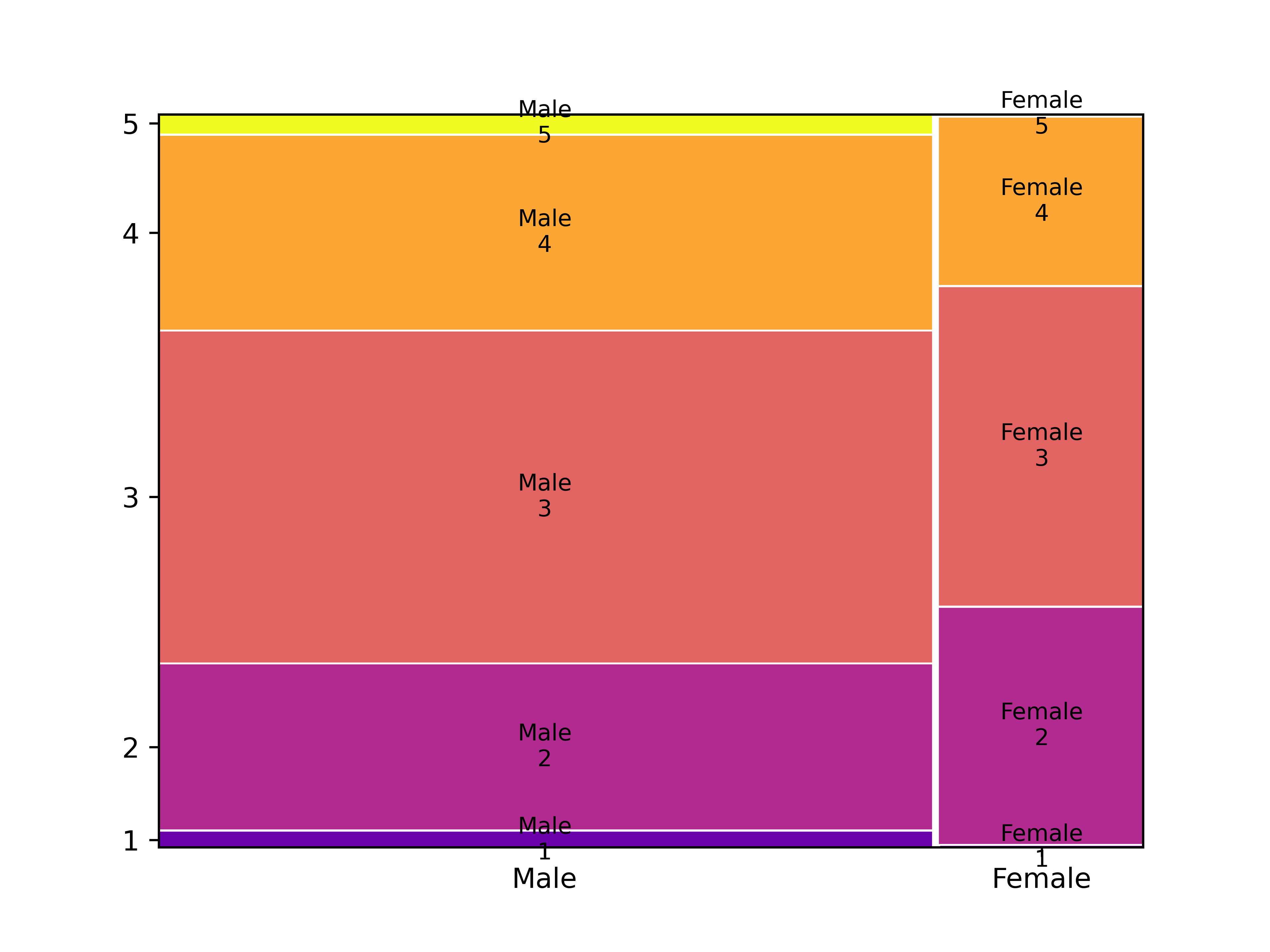

![A mosaic plot](./img/4/gender-survey-mosaic.png)

---

# Finding associations in contingency tables

-v-

## Contingency table with marginal totals

| Survey | Female | Male |  All |
| :----- | -----: | ---: | ---: |
| 1      |      0 |    4 |    4 |
| 2      |     17 |   45 |   62 |
| 3      |     23 |   91 |  114 |
| 4      |     12 |   53 |   65 |
| 5      |      0 |    5 |    5 |
| All    |     52 |  198 |  250 |

-v-

## Expected values

If there is no difference (association), we expect the same ratios in
each column of the table!

| Survey | Female |    Male |     All |
| -----: | -----: | ------: | ------: |
|      1 |  0.832 |   3.168 |   **4** |
|      2 | 12.896 |  49.104 |  **62** |
|      3 | 23.712 |  90.288 | **114** |
|      4 |  13.52 |   51.48 |  **65** |
|      5 |   1.04 |    3.96 |   **5** |
|    All | **52** | **198** | **250** |

In each cell: (row total $\times$ column total) / $n$

-v-

## Measuring dispersion

How far is the observed value $o$ from the expected $e$?

$$\frac{{(o - e)}^2}{e}$$

| Survey |    Female |       Male |
| -----: | --------: | ---------: |
|      1 |     0.832 |   0.218505 |
|      2 |   1.30605 |   0.343003 |
|      3 | 0.0213792 | 0.00561474 |
|      4 |  0.170888 |  0.0448796 |
|      5 |      1.04 |   0.273131 |

-v-

## The $\chi^2$-statistic

The sum of all these values is notated:

$$\chi^2 = \sum_i \frac{{(o_i - e_i)}^2}{e_i} \approx 4.255$$

- $\chi$ is the Greek letter *chi*
- $o_i$ = number of observations in the $i$'th cell of the contingency
  table
- $e_i$ = expected frequency

Interpretation:

- Small value $\Rightarrow$ no association
- Large value $\Rightarrow$ association

-v-

## Cramér's $V$

When is $\chi^2$ large enough?

- $2\times2$-table with $\chi^2 = 10$

- Relatively large difference

- Indicates association

- $5\times5$-table with $\chi^2 = 10$

- Relatively small difference

- Does NOT indicate association

We need a metric independent of table size!

-v-

## Cramér's V

$$V = \sqrt{\frac{\chi^2}{n(k-1)}} = \sqrt{\frac{4.255}{250(2-1)}} \approx 0.130$$

with $n$ the number of observations, $k = \min(numRows, numCols)$

Interpretation:

| Cramér's V | Interpretation          |
| :--------: | :---------------------- |
|     0      | No association          |
|    0.1     | Weak association        |
|    0.25    | Moderate association    |
|    0.50    | Strong association      |
|    0.75    | Very strong association |
|     1      | Complete association    |

---

# Chi-squared test for independence

-v-

## $\chi^2$ test for independence

- = Alternative to Cramér's V to investigate association between
  qualitative variables.

- Value of $\chi^2$ distributed according to the $\chi^2$ distribution

-v-

## The $\chi^2$ distribution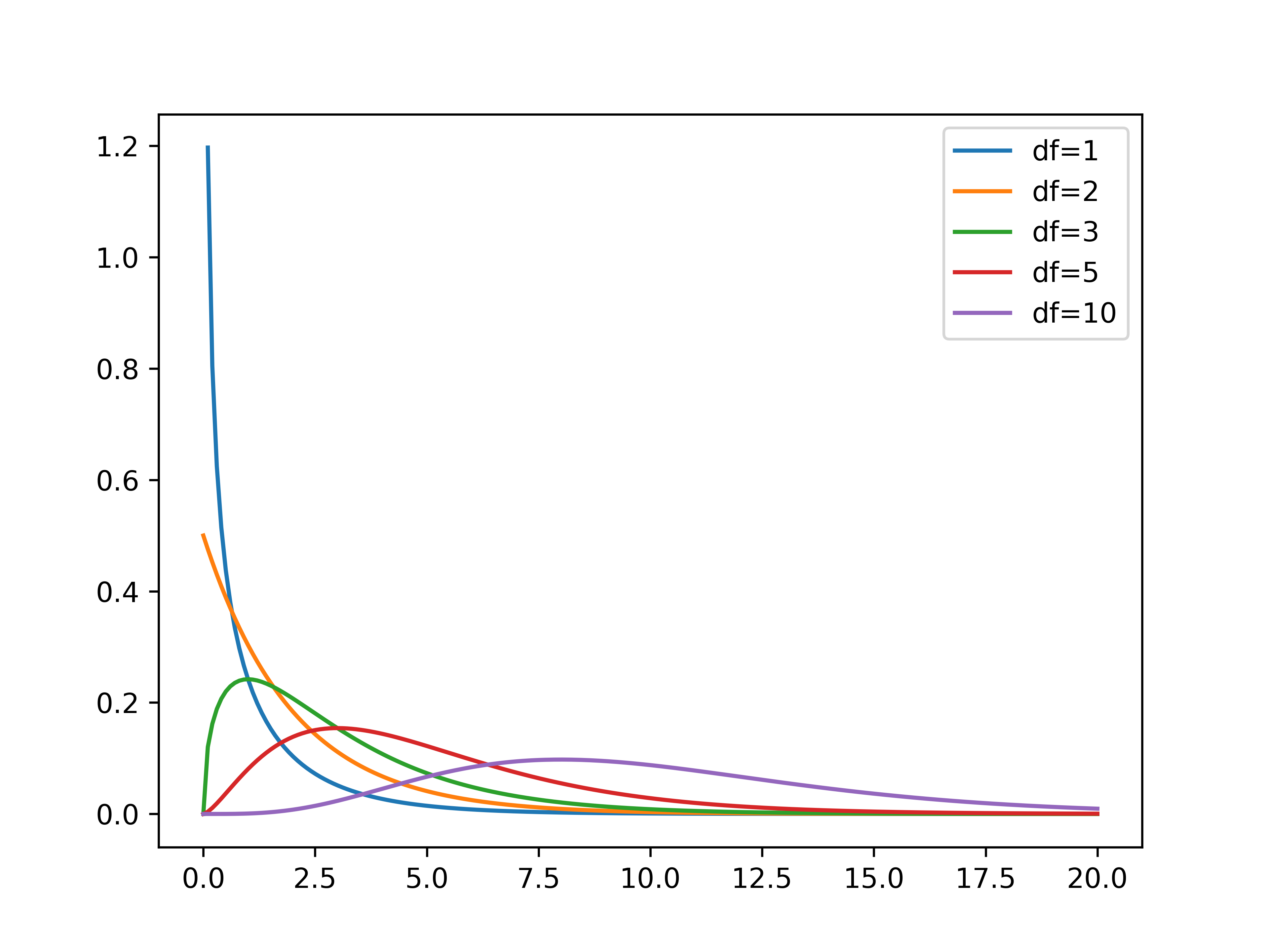

![The chi-squared distribution](./img/4/chisq-dist.png)

-v-

## $\chi^2$-distribution in Python

Import `scipy.stats`

For a $\chi^2$-distribution with `df` degrees of freedom:

-v-

## Test procedure

- **Step 1.** Formulate hypotheses:

- $H_0$: there is no association ($\chi^2$ is "small")

- $H_1$: there is an association ($\chi^2$ is "large")

- **Step 2.** Choose significance level, e.g. $\alpha = 0.05$

- **Step 3.** Calculate the test statistic, $\chi^2 = 4.255$

-v-

## Test procedure (cont.)

- **Step 4.** Use $df = (numRow-1)\times(numCol-1)$ and either:

- Determine critical value $g$ so $P(\chi^2>g)=\alpha$

- Calculate the $p$-value

- **Step 5.** Draw conclusion:

- $\chi^2 < g$: do not reject $H_0$; $\chi^2 > g$: reject $H_0$

- $p > \alpha$: do not reject $H_0$; $p < \alpha$: reject $H_0$

-v-

## Example (Gender vs Survey)

- `g = stats.chi2.isf(0.05, df=4)` (result: 9.4877)

- `p = stats.chi2.sf(4.2555, df=4)` (result: 0.3725)

![Graphical representation of the case](./img/4/chi2-test-independence.png)

-v-

## Conclusion

We do not reject the null hypothesis. Differences
between expected and observed values are not significantly large.

We found no association between variables *Gender* and *Survey*

-v-

## Test for independence in Python

SciPy has a function to calculate $\chi^2$ and $p$-value from a
contingency table:

``` python
observed = pd.crosstab(rlanders.Survey, rlanders.Gender)
chi2, p, df, expected = stats.chi2_contingency(observed)

print("Chi-squared       : %.4f" % chi2)
print("Degrees of freedom: %d" % df)
print("P-value           : %.4f" % p)
```

---

# The Goodness-of-fit test

-v-

## The Goodness-of-fit test

The $\chi^2$ test can also be used to determine whether a sample is **representative** for the population.

The **Goodness-of-fit test** indicates to what degree a sample corresponds to a null hypothesis regarding the distribution of a qualitative variable over mutually exclusive classes.

-v-

## Example

In a sample of respondents to a survey, we want to know whether the distribution of age groups is representative of the population.

```python
# Age groups=           18-25  26-35  36-45  46-55  56+
observed =   np.array([   75,    98,   127,    73,  27])
expected_p = np.array([  .17,   .23,   .35,   .17, .08])
```

Is this sample *representative* of the population? Does each age group occur in the sample in proportion to the expected percentage in the population as a whole?

-v-

## How to measure representativeness?

Is the distribution of the sample ($n = 400$) representative for the full population?

- What numbers would you *expect* if the sample is representative?

- How large are the differences from the *observed* numbers?

- small $\Rightarrow$ distribution is representative

- large $\Rightarrow$ distribution is **not** representative

Can you see the link with contingency tables and Cramer's V?

-v-

## Expected values

- Exactly representative $\Rightarrow$ 17% of respondents in age bracket 18-25
- The expected number therefore is $e = 0.35 \times 400 = 140$.

Therefore:

$$e = n \times \pi$$

If the differences $o - e$ are relatively small they can be attributed
to random sampling errors.

-v-

## Goodness of fit test

Consider $\chi^{2}$:

$$\chi^{2} = \sum_{i=1}^{n} \frac{{(o_{i} - e_{i})}^{2}}{e_{i}}$$

Draw a conclusion based on the value of $\chi^2$:

- small $\Rightarrow$ distribution is representative

- large $\Rightarrow$ distribution is **not** representative

$\chi^{2}$ measures the degree of conflict with the null hypothesis

-v-

## Goodness-of-fit test

| Age group |  $o$  | $\pi$ |  $e$  | $\frac{{(o - e)}^2}{e}$ |
| :-------: | :---: | :---: | :---: | :---------------------: |
|   18-25   |  75   | 0.17  |  68   |          0.72           |
|   26-35   |  98   | 0.23  |  92   |          0.39           |
|   36-45   |  127  | 0.35  |  140  |          1.21           |
|   46-55   |  73   | 0.17  |  68   |          0.37           |
|    56+    |  27   | 0.08  |  32   |          0.78           |
| **Total** |  400  |   1   |  400  |        **3.47**         |

-v-

## Goodness of fit test

- The test statistic $\chi^{2}$ follows the $\chi^2$ distribution with $k-1$  degrees of freedom with $k$ the number of categories.

- The critical value $g$ for a given significance level $\alpha$ and
  number of degrees of freedom `df` can be calculated in Python using
  the function `isf()`.

$$P(\chi^2 < g) = 1 - \alpha$$

-v-

## Testing procedure

- **Step 1.** Formulate hypotheses

- $H_{0}$: sample is representative for the population

- $H_{1}$: sample is not representative for the population

- **Step 2.** Choose significance level: $\alpha = 0.05$

-v-

## Testing procedure (cont.)

- **Step 3.** Calculate the test statistic $\chi^2 = 3.47$

$$\chi^{2} = \sum_{i=1}^{n} \frac{(o_{i} - e_{i})^{2}}{e_{i}}$$

- **Step 4.** Determine critical value $g$ or $p$-value

- $P(\chi^2 < g) = 1 - \alpha$
    - $p = 1 - P(X < \chi^2)$

-v-

## Testing procedure (cont.)

- **Step 5.** Draw conclusion

- $\chi^2 < g \Rightarrow$ do not reject $H_0$,

$\chi^2 > g \Rightarrow$ reject $H_0$

- $p > \alpha \Rightarrow$ do not reject $H_0$,

$p < \alpha \Rightarrow$ reject $H_0$

-v-

## Example

- `g = stats.chi2.isf(0.05, df=4)` (result: 9.4877)

- `p = stats.chi2.sf(3.4679, df=4)` (result: 0.4828)

**Conclusion.** $\chi^2 \approx 3.47 < g \approx 9.4877$, so we don't
reject the null hypothesis. This sample is representative for the
population (at least regarding the distribution of age groups).

-v-

## Goodness-of-fit test in Python

``` python
observed   = np.array([   75,    98,   127,    73,  27])
expected_p = np.array([  .17,   .23,   .35,   .17, .08])
expected   = expected_p * sum(observed)
chi2, p    = stats.chisquare(f_obs=observed, f_exp=expected)

print("χ² = %.4f" % chi2)
print("p  = %.4f" % p)
```

---

# Standardized residuals

-v-

## Example: families

Consider all families with exactly 5 children in a given community. When we look at the number of boys/girls, there are 6 possible combinations:

1. 5 boys
2. 4 boys, 1 girl
3. 3 boys, 2 girls
4. 2 boys, 3 girls
5. 1 boy, 4 girls
6. 5 girls

A survey was conducted regarding 1022 families with exactly 5 children

-v-

## Observed frequencies

|  $i$  |   0   |   1   |   2   |   3   |   4   |   5   |
| :---: | :---: | :---: | :---: | :---: | :---: | :---: |
| $o_i$ |  58   |  149  |  305  |  303  |  162  |  45   |

($i$ = number of boys)

Are the observed numbers in the 6 classes representative for a population in which the probability of having a boy is equal to the probability of having a girl, or more concrete 0.5?

-v-

## Expected frequencies

If the assumption is true, the probability $\pi_{i}$ to have $i$ boys is determined by a binomial distribution with parameters $n=5$ and $p=0.5$.

For example, the probability to have 2 boys out of 5 children is equal to:

$$(0.5)^{2} \times (1-0.5)^{5-2} \times \binom{5}{2}$$

In general (you don't have to know why):

$$\pi_{i} = \binom{5}{i}\times 0.5^{i} \times 0.5^{5-i} = \frac{5!}{i!(5-i)!}\times 0.5^{i}$$

-v-

## Summary results

|              $i$              |   0    |   1    |   2    |   3    |   4    |   5   | Total  |
| :---------------------------: | :----: | :----: | :----: | :----: | :----: | :---: | :----: |
|             $o_i$             |   58   |  149   |  305   |  303   |  162   |  45   |  1022  |
|            $\pi_i$            | 0.031  | 0.156  | 0.313  | 0.313  | 0.156  | 0.031 |   1    |
|             $e_i$             |  31.9  | 159.7  | 319.4  | 319.4  | 159.7  | 31.9  |  1022  |
| $\frac{{(o_i - e_i)}^2}{e_i}$ | 21.268 | 0.715  | 0.647  | 0.840  | 0.033  | 5.343 | 28.846 |
|             $r_i$             | 4.686  | -0.921 | -0.970 | -1.105 | -0.199 | 2.348 |        |

($r_i$ = standardized residuals, see following slides)

-v-

## Is the sample representative?

- Perform the goodness-of-fit test, for $\alpha = 0.01$.
- $\chi^2 = 28.846$ with $k-1 = 5$ degrees of freedom
- Critical value $g \approx 15.0863 < \chi^2$
- $p \approx 0.000025 < \alpha$

Conclusion: we reject the null hypothesis.

**Which categories are most problematic?**

-v-

## Standardized residuals

**Standardized Residuals** indicate which classes make the greatest contribution to the value of $\chi^2$.

$$r_{i} = \frac{o_{i} - n \pi_{i}}{\sqrt{n \pi_{i}(1-\pi_{i})}}$$

- $r_i \in [-2, 2] \Rightarrow$ "acceptable" values
- $r_i < -2 \Rightarrow$ underrepresented
- $r_i > 2 \Rightarrow$ overrepresented

**Conclusion:** families in which all children are of the same gender
are overrepresented.

---

# Cochran's rule of thumb

-v-

## Cochran's rule of thumb

In order to apply the $\chi^2$-test, the following conditions must be
met:

1. For all categories, the expected frequency $e$ must be greater than 1.

2. In a maximum of 20 % of the categories, the expected frequency $e$ may be less than 5.

If these conditions are not met, your sample is too small to apply the $\chi^2$-test. There are alternative tests, but these are not part of this course.